![]()
Introduction
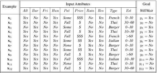
One of the simplest yet most effective forms of machine learning is decision tree induction. A decision tree takes vectors as inputs and returns a single output or “decision”. In the following article, I will discuss a decision tree classifier, implemented using sci-kit learn and vanilla python, which returns a Boolean output, e.g. “yes” or “no” answer to a question. After performing a series of tests a decision tree reaches a decision on each internal node which corresponds to a test of values from multiple attributes from a data-set. For the purposes of this demonstration I will be using a data-set found in Chapter 18 of Artificial Intelligence: A Modern Approach (3rd. Edition). The data-set consists of eleven columns and twelve rows. Our task will be to predict how likely someone is to wait for a table at a restaurant based on a series of attributes. These include whether or not there is a suitable alternative, whether there is a comfortable bar one can wait at, what type of food the restaurant is serving, in addition to seven other attributes that our decision tree classifier will take into consideration. The following image is the data-set that we will be using for our decision tree classifier:
On Decision Tree Learning
Decision trees yield concise results for a wide variety of functions, yet some functions cannot be represented so simply. To demonstration that decision trees are good for some kinds of functions but not other types of functions consider the set of all possible Boolean functions on n-attributes. The number of different functions on the set is the number of different truth tables that can be represented because a function is defined by its truth table. A truth table of n-attributes has 2^n rows, in addition, our “target” or value we are attempting to predict. e.g. WillWait, with is a 2^2^n -bit number that defines the function. All of this is an attempt to demonstrate that a 2^2^n search space is to massive for any computer to handle in a reasonable amount of time if you are working with a reasonable large data-set.
This is were some rather simple heuristics come in to reduce our tree to a small (not the smallest) consistent tree. This will allow our decision tree classifier to perform the task in a reasonable short period of time. This article gives an example of a decision tree classifier that consists of an (x, y) pair, where the x-vector is a set of attributes or features forming an input and our y-vector is a “target” column which outputs a single Boolean value of “yes” or “no” values.
A decision tree learning algorithm uses a divide-and-conquer strategy by testing the most important attributes first, which results in smaller sub-problem and recursively narrowing down into narrower sub-problems. To avoiding having to traverse an astronomically high search space the decision tree tries to find “the most important attributes” in an attempt to correctly classify our target with the smallest amount of test space given our data-set. The following image is that of a decision tree that attempts to answer the question whether or not to wait for a table.
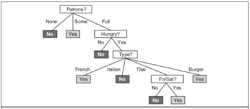
If you look closely at the table you can observe that the decision tree has no reason to include a test for Raining or Reservation, because it can classify all the examples without these attributes which results in a smaller tree.
On Information gain and Over-fitting
Now that we are aware that decision tree learning in designed in such a way to minimize the depth of our tree lets take a look at some of the concepts that decision tree learning leverage to actually make this process work. Information gain is defined in terms of the fundamental quantity found in information theory called entropy. If we take entropy to be the measure of uncertainty of a random variable, information gain can be thought of as a reduction of uncertainty. For example, if you are absolutely certain that a particular event will take place this is said to have zero entropy, on the other hand, if you flip a coin over time you will find that there is an equal likelihood that the coin will land on “heads” or “tails”. The coin flipping example has a 1-bit entropy. The following code snippet is written in python demonstrates information gain.
def gini(rows):
    """
    Gini Impurity is a measure of the likleyhood of an
    incorrect classification of a new instance of a random
    variable.
    """
    counts = class_counts(rows)
    impurity = 1
    for lbl in counts: # for labels in counts
        prob_of_lbl = counts[lbl] / float(len(rows))
        impurity -= prob_of_lbl**2
    return impurity

def info_gain(left, right, current_uncertainty):
    """
    Information gain is the reduction in entropy
    or surprise by transforming a dataset and is
    often used in training a decision trees.
    """
    p = float(len(left)) / (len(left) + len(right))
    return current_uncertainty - p * gini(left) - (1 - p) * gini(right)
Although information gain is usually a good measure for deciding the relevance for a attribute it does have its drawbacks. Problems with information gain tends to occur when it is applied to attributes which have a large value of unique values.
For example, suppose that one is building a decision tree for some data describing the customers of a business. Information gain is often used to decide which of the attributes are the most relevant, so they can be tested near the root of the tree. One of the input attributes might be the customer’s credit card number. This attribute has a high mutual information, because it uniquely identifies each customer, but we do not want to include it in the decision tree: deciding how to treat a customer based on their credit card number is unlikely to generalize to customers we haven’t seen before (over-fitting).
Therefore, when the hypothesis space and the input values get larger over-fitting tends to occurs. One way of combating this tendency is by pruning or eliminating nodes which are not likely to be relevant. This is a topic that we will come back to later.
On implementation
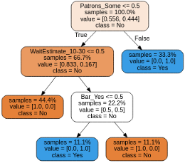
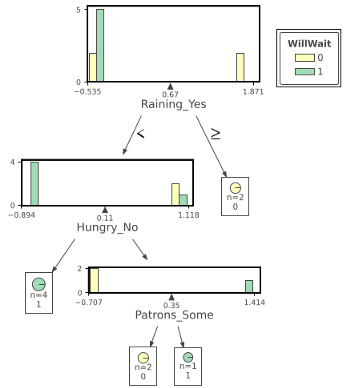
The core purpose of this article is to implement a decision tree classifier using a machine learning library, i.e. sci-kit learn, and comparing the results to a decision tree classier made from scratch using vanilla python. Sci-kit learn is a machine learning library that allows you to implement a decision tree classifier by simply importing the DecisionTreeClassifier module. After some simple pre-processing steps, e.g. categorical encoding, which changes your data into binary representations, a train test split, and some hyper-parameter tuning our model is ready for action. The entire process from begin to end takes approximately 15 minutes and produced a test accuracy of 66%. This will vary depending on your data-set and experience level. The following images give us a visual representation of what out decision tree looks like
Next, using vanilla python to implement a decision tree classifier was quite the undertaking given that it was my first attempt at coding a machine learning algorithm form scratch. Much of the rest of this article will discuss how I managed to complete the task, what I learned and how I will go about fixing some of the errors that persist in the current code base, i.e. over-fitting. I began with the notion that I could just look at the pseudo-code and code up a perfect decision tree classifier without much trouble. I quickly came to the understanding that I had not thought deeply enough about many of the concept underlying the algorithms that I have used numerous times with great success. Specifically, information gain, impurity and pruning a decision tree that is over-fitting on my data-set. Decision tree pruning combats over-fitting by cutting out the nodes that are not considered relevant. Starting from a full tree and looking at the test nodes with only one leaf as descendants, if the test appears to be irrelevant, the test is eliminated and the lead node is replaces. Something you don’t need to put much thought into if your using a machine learning library but something that was trickier than it first appears when making a decision free from scratch. Needless to say, my test accuracy was 100% which signals that additional pruning steps must be added to make the decision tree classifier fully implementable.
Conclusion
This article is probably most relevant to those who have previous experience with machine learning and consider themselves savvy enough to implement various algorithms to problems most important to them but still have some doubts about how well they understand what is going on underneath the hood. Although, I failed to produce a decision tree classifier which handles over-fitting correctly. I feel like there are some important take away’s that I feel proud of and lesson that I can carry with me into the future. First, you don’t really know an algorithm unless you can implement it from scratch using the standard python library. Yes, you might be able to import a module from your preferred machine learning library and use it to make a prediction. But understanding what is going on underneath the hood will better help you know the limitations of certain algorithm, there strengths and there weakness, and expose you to concept that are important to know as a Data Scientist, e.g. gini impurity, information gain, etc., but that you might not come across every day. Finally, although my first attempt at implementing a decision tree classifier didn’t go according to plan I feel comfortable saying I learn significantly more by failing to produce a decision tree classifier using vanilla python than by simply importing a module from sci-kit learn. P.S. I still love sci-kit learn.